SciPy：ndimage - 数理生物学演習

scipy.ndimage は，配列（格子・画像）に対するフィルター・モルフォロジカルフィルター・ラベリングなどの処理を提供する． NumPy 配列全体を1行で処理でき，自分で近傍を走査するより簡潔で高速である．拡散方程式（P2-03）や画像解析（P2-04）で用いる．

本ページでは慣例に従い次のように読み込む．

import matplotlib.pyplot as plt
import numpy as np
from scipy import ndimage as ndi

平滑化フィルター¶

gaussian_filter（ガウシアン）や uniform_filter（平均化）は，近傍の重み付き和で配列をなめらかにする．

rng = np.random.default_rng(0)
noisy = rng.random((100, 100))
smooth = ndi.gaussian_filter(noisy, sigma=3)

fig, ax = plt.subplots(1, 2, figsize=(8, 4))
ax[0].imshow(noisy, cmap="gray")
ax[0].set_title("noisy")
ax[1].imshow(smooth, cmap="gray")
ax[1].set_title("gaussian sigma=3")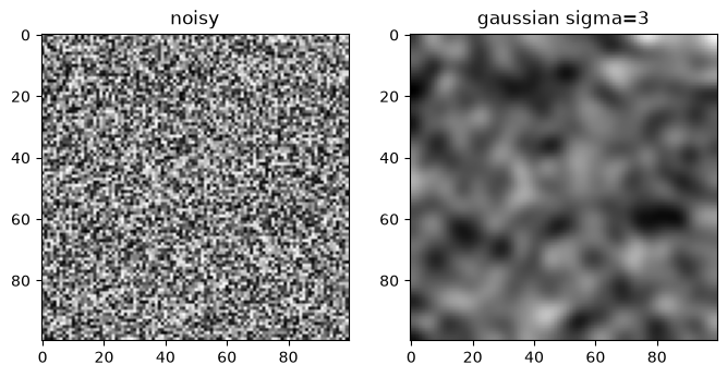

sigma（または size）を大きくするほど強く平滑化される．

畳み込み：任意のカーネル¶

convolve は，指定したカーネル（重みの小行列）と配列の畳み込み (convolution)を計算する．

kernel = np.ones((3, 3)) / 9  # 3×3 の平均化カーネル
ndi.convolve(smooth, kernel).shape

(100, 100)

微分フィルター¶

laplace（2階微分の和＝ラプラシアン (Laplacian)）や sobel（1階微分）でエッジや曲率を取り出せる．

f = np.zeros((5, 5))
f[2, 2] = 1.0  # 中央に1つだけ値を置く

# 離散ラプラシアン（上下左右の和 - 4×中央）．mode="wrap" は周期境界条件
print(ndi.laplace(f, mode="wrap"))

[[ 0.  0.  0.  0.  0.]
 [ 0.  0.  1.  0.  0.]
 [ 0.  1. -4.  1.  0.]
 [ 0.  0.  1.  0.  0.]
 [ 0.  0.  0.  0.  0.]]

mode は境界の扱いを指定する（"wrap" は周期境界，"reflect" は鏡映など）．

応用：拡散方程式¶

ラプラシアンを使うと，拡散方程式の1ステップ更新を1行で書ける（→ P2-03）．

# u の拡散による1ステップ更新（D: 拡散係数, dt: 時間刻み, dh: 空間刻み）
def diffuse(u, D, dt, dh):
    return u + D * ndi.laplace(u, mode="wrap") / dh**2 * dt


u = np.zeros((20, 20))
u[10, 10] = 100.0
for _ in range(50):
    u = diffuse(u, D=1.0, dt=0.1, dh=1.0)

plt.imshow(u)
plt.gca().set_aspect("equal")
plt.colorbar()
plt.title("diffusion via ndimage.laplace")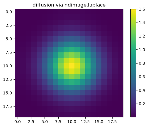

モルフォロジカルフィルター¶

二値画像の形に着目したフィルターがモルフォロジカルフィルター (morphological filter)である． binary_erosion（収縮）・binary_dilation（膨張）と，その組合せの binary_opening（オープニング）・binary_closing（クロージング）でノイズ除去や穴埋めをおこなう．

blob = np.zeros((60, 60), dtype=bool)
blob[20:40, 20:40] = True

rng = np.random.default_rng(1)
noisy_bin = (blob | (rng.random(blob.shape) < 0.03)) & ~(rng.random(blob.shape) < 0.03)
clean = ndi.binary_closing(ndi.binary_opening(noisy_bin))

fig, ax = plt.subplots(1, 2, figsize=(8, 4))
ax[0].imshow(noisy_bin, cmap="gray")
ax[0].set_title("noisy")
ax[1].imshow(clean, cmap="gray")
ax[1].set_title("opening -> closing")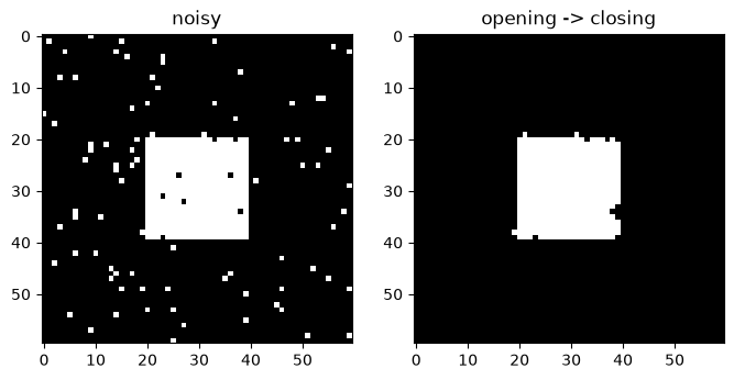

binary_fill_holes は領域内部の穴を埋める．ノイズが大きな塊のときは iterations を増やす．

ラベリング（連結成分）¶

label は，つながった前景領域に番号を振る．画像から抽出した領域の選別（P2-04）に使う．

mask = np.zeros((10, 10), dtype=bool)
mask[1:3, 1:3] = True  # 成分1
mask[5:9, 5:9] = True  # 成分2

labels, n = ndi.label(mask)
print("成分数:", n)
print(labels)

成分数: 2
[[0 0 0 0 0 0 0 0 0 0]
 [0 1 1 0 0 0 0 0 0 0]
 [0 1 1 0 0 0 0 0 0 0]
 [0 0 0 0 0 0 0 0 0 0]
 [0 0 0 0 0 0 0 0 0 0]
 [0 0 0 0 0 2 2 2 2 0]
 [0 0 0 0 0 2 2 2 2 0]
 [0 0 0 0 0 2 2 2 2 0]
 [0 0 0 0 0 2 2 2 2 0]
 [0 0 0 0 0 0 0 0 0 0]]

各成分の大きさや位置は ndi.sum や ndi.find_objects で調べられる．

拡大・縮小¶

zoom は配列を拡大・縮小する（画像のリサイズ）．

small = ndi.zoom(u, 0.5)
u.shape, small.shape

((20, 20), (10, 10))