Matplotlib（応用） - 数理生物学演習

Matplotlib の基本的な折れ線・散布図は P1-02 で扱った．ここでは Phase 2 で必要になる，2次元の場の可視化・3次元プロット・アニメーションを補う．

import matplotlib.pyplot as plt
import numpy as np

離散的な格子：matshow¶

matshow は2次元配列を格子状の画像として描く．セルオートマトン（P2-02）のような離散状態の表示に向く． cmap="binary" は 0 を白，1 を黒で表す．

rng = np.random.default_rng(0)
grid = rng.integers(0, 2, size=(20, 20))

plt.figure()
plt.matshow(grid, fignum=0, cmap="binary")
plt.title("cellular automaton state")
plt.show()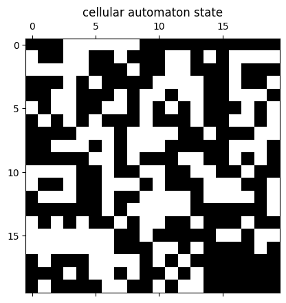

連続的な場：pcolormesh¶

pcolormesh は格子上の連続値を色で塗り分ける．拡散場（P2-03）のような連続量の表示に向く．座標格子（meshgrid）を渡すと軸が実座標になる．colorbar で色と値の対応を示す．

x = np.linspace(-3, 3, 60)
xmesh, ymesh = np.meshgrid(x, x)
u = np.exp(-(xmesh**2 + ymesh**2))

fig, ax = plt.subplots()
ax.set_aspect("equal")
pcm = ax.pcolormesh(xmesh, ymesh, u, vmin=0, vmax=1)
fig.colorbar(pcm, ax=ax, shrink=0.8)
plt.show()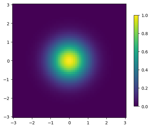

3次元曲面：plot_surface¶

3次元曲面は mplot3d で描く．add_subplot(projection="3d") で3次元の軸を作り，plot_surface に格子を渡す．

from mpl_toolkits.mplot3d import Axes3D  # noqa: F401  (3D 投影の登録に必要)

fig = plt.figure(figsize=(7, 5))
ax = fig.add_subplot(111, projection="3d")
surf = ax.plot_surface(xmesh, ymesh, u, vmin=0, vmax=1)
fig.colorbar(surf, shrink=0.7)
plt.show()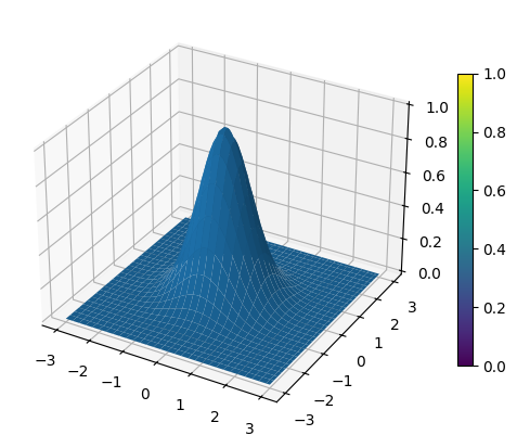

アニメーション（フォールバック）¶

時間発展の可視化は Plotly を標準とするが，Matplotlib でもアニメーションを作れる． ArtistAnimation に各フレームの描画オブジェクトのリストを渡し，jshtml 形式で表示すると，Web ページ上でも再生できる JavaScript アニメーションになる．

from matplotlib import animation, rc
from IPython.display import HTML  # noqa: F401

# 各時刻の場（広がるガウス分布）を作る
fields = [
    np.exp(-(xmesh**2 + ymesh**2) / (2 * t**2)) for t in np.linspace(0.3, 2.5, 20)
]

fig, ax = plt.subplots()
plt.close()  # 静止画の二重表示を防ぐ
ax.set_aspect("equal")

artists = []
for f in fields:
    im = ax.pcolormesh(xmesh, ymesh, f, vmin=0, vmax=1)
    artists.append([im])

ani = animation.ArtistAnimation(fig, artists, interval=100)
rc("animation", html="jshtml")
ani

フレーム数が多いと出力が重くなるため，記録する時刻を間引くとよい．