輪郭抽出
二値化とモルフォロジカルフィルターを組み合わせ,葉の輪郭を座標として取り出す.
import urllib.request

import matplotlib.pyplot as plt
import numpy as np
from matplotlib.colors import rgb_to_hsv
from scipy import ndimage as ndi
base = "https://assets.ku-compbio.noshita.net/2026/P2-04/images/"
filename = "Pedu1_1_4.png"
urllib.request.urlretrieve(base + filename, filename)
img = plt.imread(filename)[:, :, :3]
img_gray = img @ [0.2989, 0.587, 0.114]
plt.imshow(img)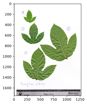
03-01. 二値化と閾値処理
画像を前景(葉)と背景に分ける処理が二値化 (binarization)である. まず輝度ヒストグラムを見て,閾値の見当をつける.
plt.hist(img_gray.ravel(), bins=256)(array([1.00000e+01, 4.50000e+01, 3.60000e+01, 4.10000e+01, 9.50000e+01,
3.97000e+02, 1.75000e+02, 9.50000e+01, 1.41000e+02, 1.64000e+02,
1.83000e+02, 2.37000e+02, 6.14000e+02, 1.29100e+03, 2.62800e+03,
3.37200e+03, 2.71200e+03, 2.61500e+03, 2.53100e+03, 2.71000e+03,
2.49000e+03, 2.46800e+03, 2.19800e+03, 1.97100e+03, 1.68800e+03,
1.69200e+03, 1.43000e+03, 1.35000e+03, 1.27500e+03, 1.20400e+03,
1.15400e+03, 1.02000e+03, 1.05600e+03, 9.47000e+02, 8.68000e+02,
8.47000e+02, 7.73000e+02, 7.67000e+02, 7.55000e+02, 6.85000e+02,
7.03000e+02, 6.26000e+02, 6.23000e+02, 5.85000e+02, 5.95000e+02,
6.04000e+02, 5.73000e+02, 5.74000e+02, 5.33000e+02, 5.64000e+02,
5.71000e+02, 5.41000e+02, 5.83000e+02, 5.95000e+02, 5.99000e+02,
6.16000e+02, 6.67000e+02, 6.71000e+02, 7.08000e+02, 7.36000e+02,
7.61000e+02, 8.62000e+02, 9.39000e+02, 9.63000e+02, 1.03000e+03,
9.97000e+02, 1.12700e+03, 1.10400e+03, 1.22000e+03, 1.28700e+03,
1.35900e+03, 1.46400e+03, 1.53300e+03, 1.57400e+03, 1.75300e+03,
1.84100e+03, 1.92600e+03, 2.15400e+03, 2.22700e+03, 2.40300e+03,
2.42600e+03, 2.52100e+03, 2.79500e+03, 2.84900e+03, 3.00000e+03,
3.05900e+03, 3.26500e+03, 3.29600e+03, 3.37400e+03, 3.62700e+03,
3.72200e+03, 3.87800e+03, 4.00300e+03, 4.08800e+03, 4.25100e+03,
4.44200e+03, 4.64400e+03, 4.81800e+03, 4.90900e+03, 5.09300e+03,
5.34100e+03, 5.50700e+03, 5.91000e+03, 6.13400e+03, 6.27800e+03,
6.44300e+03, 6.94600e+03, 7.19000e+03, 7.36900e+03, 7.87000e+03,
7.95300e+03, 8.19300e+03, 8.54300e+03, 8.94100e+03, 9.45000e+03,
9.62600e+03, 9.90700e+03, 1.04400e+04, 1.05810e+04, 1.11320e+04,
1.11360e+04, 1.13880e+04, 1.15400e+04, 1.17800e+04, 1.19620e+04,
1.16380e+04, 1.16960e+04, 1.15910e+04, 1.15980e+04, 1.11690e+04,
1.11060e+04, 1.07780e+04, 1.02820e+04, 1.02790e+04, 9.97800e+03,
9.68000e+03, 9.44800e+03, 9.01600e+03, 8.80400e+03, 8.51100e+03,
8.42300e+03, 8.21800e+03, 7.97000e+03, 7.68900e+03, 7.59300e+03,
7.22300e+03, 6.82400e+03, 6.67600e+03, 6.27200e+03, 5.85500e+03,
5.53000e+03, 5.29700e+03, 4.80300e+03, 4.57200e+03, 4.27600e+03,
3.93700e+03, 3.71100e+03, 3.31100e+03, 3.15300e+03, 2.79500e+03,
2.60700e+03, 2.47000e+03, 2.47600e+03, 2.28500e+03, 2.32100e+03,
2.26500e+03, 2.32600e+03, 2.24100e+03, 2.32700e+03, 2.32600e+03,
2.51700e+03, 2.56400e+03, 2.58900e+03, 2.54400e+03, 2.52100e+03,
2.50800e+03, 2.33800e+03, 2.14000e+03, 2.03900e+03, 1.91400e+03,
1.83500e+03, 1.72100e+03, 1.68600e+03, 1.69200e+03, 1.77800e+03,
1.79700e+03, 2.01100e+03, 2.18600e+03, 2.50300e+03, 2.81200e+03,
3.51700e+03, 3.65800e+03, 4.15200e+03, 4.37300e+03, 4.62000e+03,
4.29600e+03, 4.17500e+03, 3.62400e+03, 3.03900e+03, 2.31400e+03,
1.84400e+03, 1.28400e+03, 8.96000e+02, 7.18000e+02, 4.92000e+02,
4.61000e+02, 4.13000e+02, 3.71000e+02, 3.39000e+02, 3.53000e+02,
3.70000e+02, 3.85000e+02, 3.69000e+02, 3.49000e+02, 3.84000e+02,
3.31000e+02, 3.28000e+02, 3.43000e+02, 3.08000e+02, 3.09000e+02,
2.98000e+02, 3.48000e+02, 3.65000e+02, 3.84000e+02, 4.65000e+02,
4.08000e+02, 4.43000e+02, 4.57000e+02, 4.50000e+02, 4.96000e+02,
5.04000e+02, 5.21000e+02, 6.08000e+02, 6.07000e+02, 6.21000e+02,
6.59000e+02, 6.34000e+02, 7.00000e+02, 7.13000e+02, 7.63000e+02,
7.73000e+02, 8.16000e+02, 9.40000e+02, 1.04000e+03, 1.09300e+03,
1.32500e+03, 1.54000e+03, 1.95200e+03, 2.39200e+03, 3.49600e+03,
6.51500e+03, 2.26300e+04, 3.62420e+04, 1.16802e+05, 3.38744e+05,
9.05123e+05]),
array([0.00481529, 0.00870234, 0.01258939, 0.01647644, 0.02036349,
0.02425054, 0.02813759, 0.03202464, 0.03591169, 0.03979874,
0.04368579, 0.04757284, 0.05145989, 0.05534694, 0.05923399,
0.06312104, 0.06700809, 0.07089514, 0.07478219, 0.07866924,
0.08255629, 0.08644334, 0.09033039, 0.09421744, 0.09810449,
0.10199154, 0.10587858, 0.10976563, 0.11365268, 0.11753973,
0.12142678, 0.12531383, 0.12920088, 0.13308793, 0.13697498,
0.14086203, 0.14474908, 0.14863613, 0.15252318, 0.15641023,
0.16029728, 0.16418433, 0.16807138, 0.17195843, 0.17584548,
0.17973253, 0.18361958, 0.18750663, 0.19139368, 0.19528073,
0.19916778, 0.20305483, 0.20694188, 0.21082892, 0.21471597,
0.21860302, 0.22249007, 0.22637712, 0.23026417, 0.23415122,
0.23803827, 0.24192532, 0.24581237, 0.24969942, 0.25358647,
0.25747352, 0.26136057, 0.26524762, 0.26913467, 0.27302172,
0.27690877, 0.28079582, 0.28468287, 0.28856992, 0.29245697,
0.29634402, 0.30023107, 0.30411812, 0.30800517, 0.31189222,
0.31577926, 0.31966631, 0.32355336, 0.32744041, 0.33132746,
0.33521451, 0.33910156, 0.34298861, 0.34687566, 0.35076271,
0.35464976, 0.35853681, 0.36242386, 0.36631091, 0.37019796,
0.37408501, 0.37797206, 0.38185911, 0.38574616, 0.38963321,
0.39352026, 0.39740731, 0.40129436, 0.40518141, 0.40906846,
0.41295551, 0.41684256, 0.4207296 , 0.42461665, 0.4285037 ,
0.43239075, 0.4362778 , 0.44016485, 0.4440519 , 0.44793895,
0.451826 , 0.45571305, 0.4596001 , 0.46348715, 0.4673742 ,
0.47126125, 0.4751483 , 0.47903535, 0.4829224 , 0.48680945,
0.4906965 , 0.49458355, 0.4984706 , 0.50235765, 0.5062447 ,
0.51013175, 0.5140188 , 0.51790585, 0.5217929 , 0.52567994,
0.52956699, 0.53345404, 0.53734109, 0.54122814, 0.54511519,
0.54900224, 0.55288929, 0.55677634, 0.56066339, 0.56455044,
0.56843749, 0.57232454, 0.57621159, 0.58009864, 0.58398569,
0.58787274, 0.59175979, 0.59564684, 0.59953389, 0.60342094,
0.60730799, 0.61119504, 0.61508209, 0.61896914, 0.62285619,
0.62674324, 0.63063029, 0.63451733, 0.63840438, 0.64229143,
0.64617848, 0.65006553, 0.65395258, 0.65783963, 0.66172668,
0.66561373, 0.66950078, 0.67338783, 0.67727488, 0.68116193,
0.68504898, 0.68893603, 0.69282308, 0.69671013, 0.70059718,
0.70448423, 0.70837128, 0.71225833, 0.71614538, 0.72003243,
0.72391948, 0.72780653, 0.73169358, 0.73558063, 0.73946767,
0.74335472, 0.74724177, 0.75112882, 0.75501587, 0.75890292,
0.76278997, 0.76667702, 0.77056407, 0.77445112, 0.77833817,
0.78222522, 0.78611227, 0.78999932, 0.79388637, 0.79777342,
0.80166047, 0.80554752, 0.80943457, 0.81332162, 0.81720867,
0.82109572, 0.82498277, 0.82886982, 0.83275687, 0.83664392,
0.84053097, 0.84441801, 0.84830506, 0.85219211, 0.85607916,
0.85996621, 0.86385326, 0.86774031, 0.87162736, 0.87551441,
0.87940146, 0.88328851, 0.88717556, 0.89106261, 0.89494966,
0.89883671, 0.90272376, 0.90661081, 0.91049786, 0.91438491,
0.91827196, 0.92215901, 0.92604606, 0.92993311, 0.93382016,
0.93770721, 0.94159426, 0.94548131, 0.94936835, 0.9532554 ,
0.95714245, 0.9610295 , 0.96491655, 0.9688036 , 0.97269065,
0.9765777 , 0.98046475, 0.9843518 , 0.98823885, 0.9921259 ,
0.99601295, 0.9999 ]),
<BarContainer object of 256 artists>)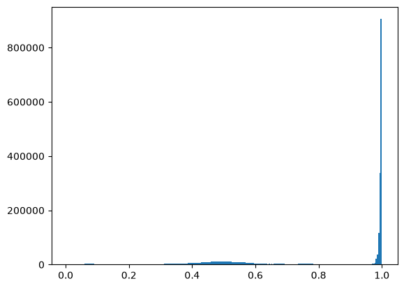
背景の白い(明るい)画素が多い.閾値より暗い画素を前景とする.
img_bin = img_gray < 0.7
plt.imshow(img_bin, cmap="gray")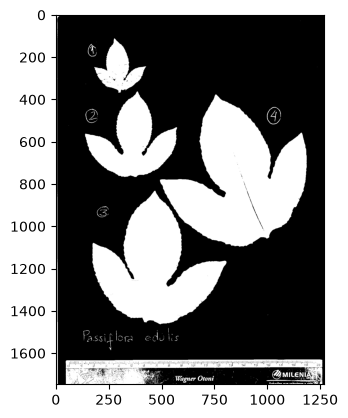
葉は取れるが,下部の定規や手書きの文字も拾ってしまっている.
03-02. 大津の二値化
閾値を手で決める代わりに,大津の二値化 (Otsu's method)はヒストグラムから 前景と背景のクラス間分散が最大になる値を自動で選ぶ.数行で実装できる.
def otsu_threshold(gray, nbins=256):
    """輝度ヒストグラムからクラス間分散が最大となる閾値を返す."""
    hist, edges = np.histogram(gray.ravel(), bins=nbins, range=(0.0, 1.0))
    centers = (edges[:-1] + edges[1:]) / 2
    weight0 = np.cumsum(hist)  # 閾値以下の画素数
    weight1 = weight0[-1] - weight0  # 閾値より上の画素数
    sum0 = np.cumsum(hist * centers)
    mean0 = np.divide(sum0, weight0, out=np.zeros(nbins), where=weight0 > 0)
    mean1 = np.divide(sum0[-1] - sum0, weight1, out=np.zeros(nbins), where=weight1 > 0)
    var_between = weight0 * weight1 * (mean0 - mean1) ** 2
    return centers[np.argmax(var_between)]


t = otsu_threshold(img_gray)
tnp.float64(0.720703125)plt.imshow(img_gray < t, cmap="gray")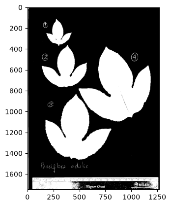
自動で閾値が決まったが,輝度だけでは定規や文字を葉と区別できない.
03-03. 色による分離
葉は緑,定規は灰色,文字は青である. HSV 色空間の色相(hue)で緑だけを選べば,葉を分離できる.
hsv = rgb_to_hsv(img)
hue = hsv[:, :, 0]
sat = hsv[:, :, 1]

# 緑色相(およそ 0.05〜0.55)かつ彩度のある画素.厳しくすると葉の基部が削れるため広めにとる
green = (hue > 0.05) & (hue < 0.55) & (sat > 0.06)
plt.imshow(green, cmap="gray")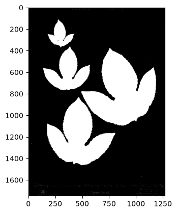
定規・文字が消え,葉だけが残った.
03-04. 二値画像の整形
モルフォロジカルフィルターで細かなノイズを除き,葉の内部の穴を埋める.
leaf = ndi.binary_opening(green)  # 細かなノイズを除去(強すぎると葉の基部が削れる)
leaf = ndi.binary_fill_holes(leaf)  # 内部の穴を埋める
plt.imshow(leaf, cmap="gray")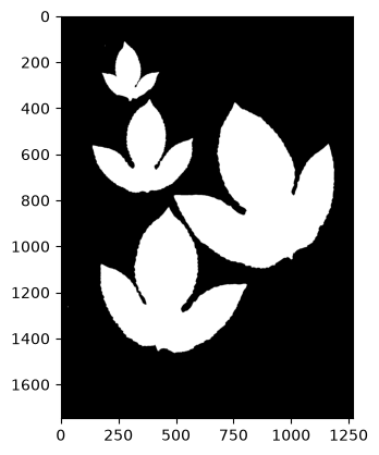
03-05. 輪郭抽出
二値画像の境界を輪郭 (contour)として取り出す.
plt.contour は値が 0.5 を横切る線(マーチングスクエア法)を,順序付きの座標として返す.
fig, ax = plt.subplots()
ax.imshow(img)
cs = ax.contour(leaf, levels=[0.5], colors="red", linewidths=1.5)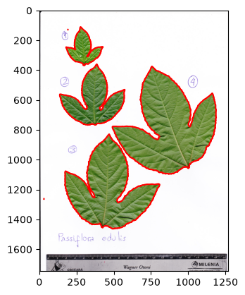
contours = cs.allsegs[0]  # 各輪郭は (N, 2) の (x, y) 座標
len(contours)6葉の枚数だけ輪郭が得られた.
03-06. 輪郭の選別
Shoelace formula で各輪郭が囲む面積を求め,小さすぎる輪郭を除いて葉の輪郭だけを残す.
def shoelace_area(xy):
    """順序付き座標 (N, 2) が囲む多角形の面積(Shoelace formula)."""
    x, y = xy[:, 0], xy[:, 1]
    return 0.5 * abs(np.dot(x, np.roll(y, -1)) - np.dot(y, np.roll(x, -1)))


min_area = 0.005 * leaf.size
leaf_contours = [c for c in contours if shoelace_area(c) > min_area]
[int(shoelace_area(c)) for c in leaf_contours]
[29405, 87563, 275726, 204162]fig, ax = plt.subplots()
ax.imshow(img)
for c in leaf_contours:
ax.plot(c[:, 0], c[:, 1], "r-", lw=1.5)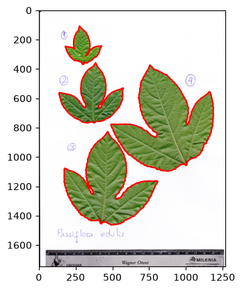
各葉の輪郭が座標データとして得られた.
03-07. 形態測定への接続
取り出した輪郭座標は,葉の「かたち」を表す数値データである. 最も大きい葉の輪郭を1枚取り出して描いてみよう.
biggest = max(leaf_contours, key=shoelace_area)
plt.plot(biggest[:, 0], -biggest[:, 1])  # 画像座標に合わせて y を反転
plt.axis("equal")
(np.float64(455.6),
np.float64(1223.4),
np.float64(-1132.6),
np.float64(-338.4))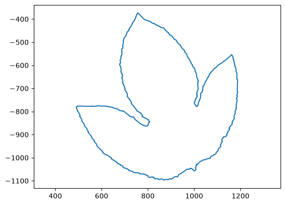
複数の画像・複数の種から輪郭を集めれば,形態を定量的に比較できる(manifest.csv に5種を収録).
輪郭を楕円フーリエ解析などで数値化すると,種間・個体間の形態差を統計的に扱える.
これが形態測定学 (morphometrics)の出発点であり,P2-01 理論形態学のかたちの数理モデルとつながる.
Solution to Exercise 1
fn2 = "Pcin1_1_6.png"
urllib.request.urlretrieve(base + fn2, fn2)
img2 = plt.imread(fn2)[:, :, :3]

hsv2 = rgb_to_hsv(img2)
green2 = (hsv2[:, :, 0] > 0.05) & (hsv2[:, :, 0] < 0.55) & (hsv2[:, :, 1] > 0.06)
leaf2 = ndi.binary_fill_holes(ndi.binary_opening(green2))

fig, ax = plt.subplots()
cs2 = ax.contour(leaf2, levels=[0.5])
plt.close(fig)

contours2 = [c for c in cs2.allsegs[0] if shoelace_area(c) > 0.005 * leaf2.size]
print("葉の枚数:", len(contours2))
print("面積:", [int(shoelace_area(c)) for c in contours2])
葉の枚数: 6
面積: [88776, 37690, 70130, 97895, 89294, 151340]