フィルターによる画像処理

フィルターによる画像処理を学ぶ．

import urllib.request

import matplotlib.pyplot as plt
import numpy as np
from scipy import ndimage as ndi

# 前章と同じ葉画像をグレイスケールで用意する
base = "https://assets.ku-compbio.noshita.net/2026/P2-04/images/"
filename = "Pedu1_1_4.png"
urllib.request.urlretrieve(base + filename, filename)

img = plt.imread(filename)
img_gray = img[:, :, :3] @ [0.2989, 0.587, 0.114]
plt.imshow(img_gray, cmap="gray")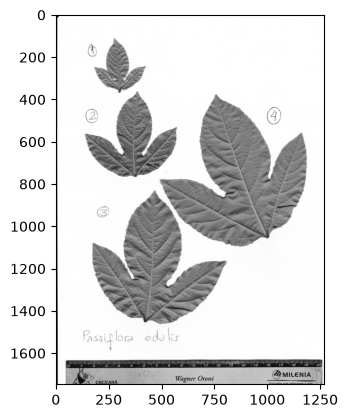

02-01. 畳み込みとカーネル¶

フィルター処理の多くは畳み込み (convolution)で表される．画素の近傍にカーネル (kernel)（重みの小さな行列）を掛けて和をとる操作である．

# 3×3 の平均化カーネル
kernel = np.ones((3, 3)) / 9
kernel

array([[0.11111111, 0.11111111, 0.11111111],
       [0.11111111, 0.11111111, 0.11111111],
       [0.11111111, 0.11111111, 0.11111111]])

img_mean = ndi.convolve(img_gray, kernel)
plt.imshow(img_mean, cmap="gray")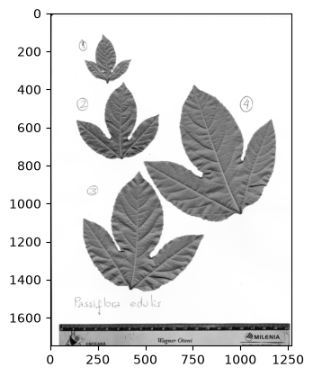

微分を差分で近似するのと同じく，カーネルを変えればぼかし・微分・先鋭化など様々な操作を表せる（有限差分法）．

02-02. 平滑化¶

画像をぼかすと細かなノイズが減り，後段の二値化・輪郭抽出が安定する．

img_g3 = ndi.gaussian_filter(img_gray, sigma=3)
img_g6 = ndi.gaussian_filter(img_gray, sigma=6)

fig, axes = plt.subplots(1, 3, figsize=(14, 5))
for ax, im, title in zip(
    axes, [img_gray, img_g3, img_g6], ["original", "gaussian sigma=3", "gaussian sigma=6"]
):
    ax.imshow(im, cmap="gray")
    ax.set_title(title)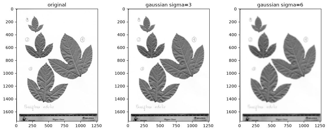

sigma を大きくするほど強くぼける．単純な平均化は ndi.uniform_filter でもおこなえる．

02-03. 微分フィルターとエッジ検出¶

輝度が急に変わる境界，すなわちエッジは輝度の微分で取り出せる（エッジ検出 (edge detection)）．

# ラプラシアン（2階微分）．先にぼかしてノイズを抑える
img_lap = ndi.laplace(ndi.gaussian_filter(img_gray, 3))
plt.imshow(img_lap, cmap="gray")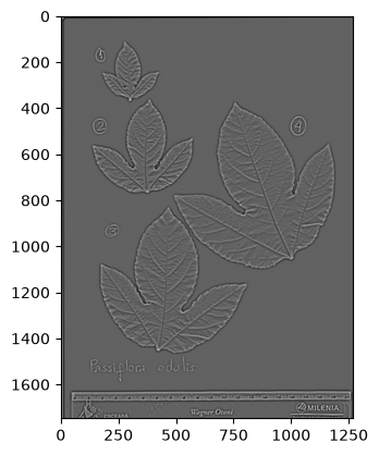

ラプラシアン (Laplacian)は2階微分の和で輪郭を強調する． 1階微分の Sobel フィルターでは，方向ごとの勾配が得られる．

sobel_y = ndi.sobel(img_gray, axis=0)  # 縦方向の勾配
sobel_x = ndi.sobel(img_gray, axis=1)  # 横方向の勾配
grad = np.hypot(sobel_x, sobel_y)  # 勾配の大きさ

fig, axes = plt.subplots(1, 3, figsize=(14, 5))
for ax, im, title in zip(
    axes, [sobel_x, sobel_y, grad], ["Sobel x", "Sobel y", "gradient magnitude"]
):
    ax.imshow(im, cmap="gray")
    ax.set_title(title)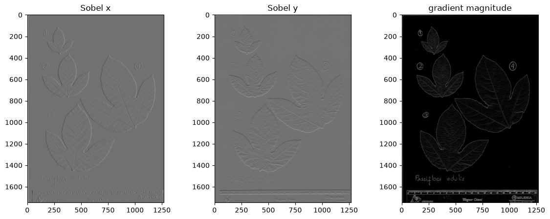

勾配の大きさはエッジを明瞭に示す．より洗練されたエッジ検出として Canny 法などがある．

02-04. モルフォロジカルフィルター¶

二値画像の形に着目したフィルターをモルフォロジカルフィルター (morphological filter)という．収縮・膨張とその組合せでノイズを除去できる．

# 合成した二値画像にノイズを加える
blob = np.zeros((120, 120), dtype=bool)
blob[30:90, 30:90] = True

rng = np.random.default_rng(0)
salt = rng.random(blob.shape) < 0.03  # 背景の白ノイズ
pepper = rng.random(blob.shape) < 0.03  # 前景の黒ノイズ
noisy = (blob | salt) & ~(pepper & blob)

plt.imshow(noisy, cmap="gray")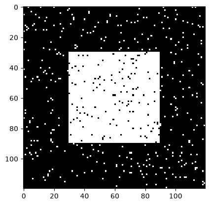

まず基本となる収縮（erosion）と膨張（dilation）を見る．

eroded = ndi.binary_erosion(noisy)
dilated = ndi.binary_dilation(noisy)

fig, axes = plt.subplots(1, 2, figsize=(8, 4))
for ax, im, title in zip(axes, [eroded, dilated], ["erosion", "dilation"]):
    ax.imshow(im, cmap="gray")
    ax.set_title(title)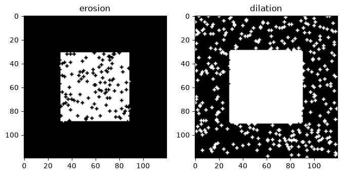

収縮と膨張を組み合わせたのがオープニング（opening）とクロージング（closing）である．それぞれ一方のノイズにだけ効き，オープニングは背景の点を，クロージングは前景の穴を除去する．

opened = ndi.binary_opening(noisy)  # オープニング（収縮→膨張）
closed = ndi.binary_closing(noisy)  # クロージング（膨張→収縮）

fig, axes = plt.subplots(1, 2, figsize=(8, 4))
for ax, im, title in zip(axes, [opened, closed], ["opening", "closing"]):
    ax.imshow(im, cmap="gray")
    ax.set_title(title)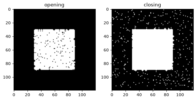

オープニングでは背景の点が消え（前景の穴は残る），クロージングでは前景の穴が埋まる（背景の点は残る）．

大きなノイズを消すにはカーネルを大きくする．iterations で収縮・膨張を繰り返すと，より大きなノイズも除去できる．

# 大小のノイズを含む二値画像（正方形は塗りつぶし）
salt_big = (rng.random(blob.shape) < 0.02) | ndi.binary_dilation(
    rng.random(blob.shape) < 0.0015, iterations=2
)
noisy_salt = blob | salt_big

op1 = ndi.binary_opening(noisy_salt, iterations=1)  # 小さな白い点のみ除去
op3 = ndi.binary_opening(noisy_salt, iterations=3)  # 大きな白い点も除去

fig, axes = plt.subplots(1, 3, figsize=(12, 4))
for ax, im, title in zip(
    axes, [noisy_salt, op1, op3], ["salt only", "opening iterations=1", "opening iterations=3"]
):
    ax.imshow(im, cmap="gray")
    ax.set_title(title)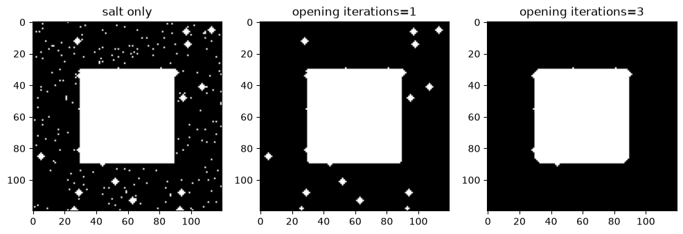

iterations を上げるほど（カーネルが大きいほど），より大きなノイズも除去できる．ただし，逆に構造の詳細が崩れやすい．次章では，これを二値化した後の整形に使う．

Solution to Exercise 1

sharpen = np.array([[0, -1, 0], [-1, 5, -1], [0, -1, 0]])
img_sharp = ndi.convolve(img_gray, sharpen)
plt.imshow(img_sharp, cmap="gray")