1次元セル・オートマトン
1次元セル・オートマトン
ここでは2状態1次元1近傍セル・オートマトンを考える. 以下の仮定を置く.
仮定
セルが1次元的に並んでいる
セルは状態0または1のいずれかをもつ
セルは自身と近傍の状態により次のステップでの状態が決まる
ある時間ステップ でのセルの配列を横1列に並べ, の状態をその下に記録していくと,横軸が空間(セルの位置),縦軸が時間(ステップ数)の図を描写できる. シンプルなルールから複雑なパターンが生み出されるセル・オートマトンの振る舞いが,この図により可視化される.
<Figure size 1920x1440 with 0 Axes>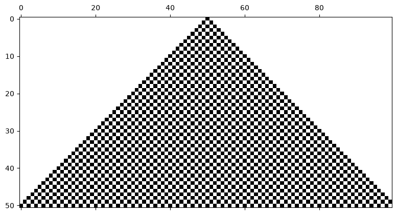
2状態1次元1近傍セルオートマトンのルールの命名規則
自身と近傍の状態は8通り.
自身と近傍の状態に対して,0または1の2通りに遷移する可能性がある.
よって,遷移ルールの総数は28通り.
以下の命名規則を採用する.
2進法で各桁を(1, 1, 1)〜(0, 0, 0)に対応させ遷移後の状態を各桁の値とする
その10進数表示をルール名とする
たとえば,8通りの出力が であれば, 2進数で 10110010 となり,
このルールは「ルール178」と呼ばれる.
ルール178の実装
まずはシンプルにifで条件分岐させることで,ルール178を実装してみる.
# ルール178
def rule178(cell1, cell2, cell3):
    if cell1 == 0:
        if cell2 == 0:
            if cell3 == 0:
                return 0
            elif cell3 == 1:
                return 1
        elif cell2 == 1:
            if cell3 == 0:
                return 0
            elif cell3 == 1:
                return 0
    elif cell1 == 1:
        if cell2 == 0:
            if cell3 == 0:
                return 1
            elif cell3 == 1:
                return 1
        elif cell2 == 1:
            if cell3 == 0:
                return 0
            elif cell3 == 1:
return 1cell1(左),cell2(中央),cell1(右)のセルの状態を引数で渡し,中央の次のステップの状態が返ってくる.
# 確認
for cell1 in range(2):
    for cell2 in range(2):
        for cell3 in range(2):
            print(cell1, cell2, cell3, ": ", rule178(cell1, cell2, cell3))
0 0 0 : 0
0 0 1 : 1
0 1 0 : 0
0 1 1 : 0
1 0 0 : 1
1 0 1 : 1
1 1 0 : 0
1 1 1 : 1
これを使ってセル・オートマトンを実行しよう.
セルを100個ならべ,真ん中に一つだけ1,それ以外は0を初期値として,50ステップ計算してみる.
# セルオートマトンの実行
# パッケージの読み込み等
import numpy as np
import matplotlib.pyplot as plt

num_cell = 100  # セルの数
steps = 50  # 何ステップまで計算するか

cell_list = []  # 各世代のセルの情報を記録するリスト
cell = np.zeros(num_cell, dtype=int)  # セルの初期化

cell[int(num_cell / 2)] = 1  # 一つのセルだけに1を代入
cell_list.append(cell)
for t in range(steps):
    # -- 状態遷移 --
    cell_tmp = np.ones(num_cell, dtype=int)
    # 境界条件処理その1
    cell_tmp[0] = rule178(cell[num_cell - 1], cell[0], cell[1])
    # メイン
    for i in range(1, num_cell - 1, 1):
        cell_tmp[i] = rule178(cell[i - 1], cell[i], cell[i + 1])
    # 境界条件処理その2
    cell_tmp[num_cell - 1] = rule178(cell[num_cell - 2], cell[num_cell - 1], cell[0])

    # 情報の更新
    cell = np.copy(cell_tmp)
cell_list.append(cell)cell_listに各世代のセルの状態が記録されていく.
# セルオートマトンの可視化
plt.figure(dpi=300)
plt.matshow(cell_list[:], cmap="binary")
<Figure size 1920x1440 with 0 Axes>最後はmatshowを使って可視化しよう.二値(0か1)なのでcmap="binaryとする.
境界条件
空間構造を扱う場合は,「端」の処理に注意が必要. 1次元セル・オートマトンでは,最も左のセルには「左近傍」が,最も右のセルには「右近傍」が存在しないため, 何らかの仮定を置く必要がある.これを境界条件という.
周期境界条件と固定端境界条件が良く利用される. 周期境界条件では,左端と右端が繋がっていると考える(左端のセルの左近傍は右端のセル,右端のセルの右近傍は左端のセル). 1次元の場合,これはセルが円環状に並んでいるとみなすことに相当する.
固定端境界条件では,端のセルの値をあらかじめ固定して変動しない. 両端を常に一定の状態(例えば0)に保つ.
上のシミュレーションではでは周期境界条件を採用している. 左端(インデックス 0)の左近傍としてインデックス (最後のセル)を, 右端(インデックス )の右近傍としてインデックス 0(最初のセル)を参照している.
別のルールの実装
その他のルールも実装して,シミュレーションしてみよう.
ルール0(クラス1)
Solution to Exercise 1
すべての場合で0を返せば良い.
# ルール0
def rule0(cell1, cell2, cell3):
    if cell1 == 0:
        if cell2 == 0:
            if cell3 == 0:
                return 0
            elif cell3 == 1:
                return 0
        elif cell2 == 1:
            if cell3 == 0:
                return 0
            elif cell3 == 1:
                return 0
    elif cell1 == 1:
        if cell2 == 0:
            if cell3 == 0:
                return 0
            elif cell3 == 1:
                return 0
        elif cell2 == 1:
            if cell3 == 0:
                return 0
            elif cell3 == 1:
return 0rule0を使って同様にシミュレーションしてみよう.
num_cell = 100
steps = 50

cell_list = []
cell = np.zeros(num_cell, dtype=int)

cell[int(num_cell / 2)] = 1
cell_list.append(cell)
for t in range(steps):
    # -- 状態遷移 --
    cell_tmp = np.ones(num_cell, dtype=int)
    # 境界条件処理その1
    cell_tmp[0] = rule0(cell[num_cell - 1], cell[0], cell[1])
    # メイン
    for i in range(1, num_cell - 1, 1):
        cell_tmp[i] = rule0(cell[i - 1], cell[i], cell[i + 1])
    # 境界条件処理その2
    cell_tmp[num_cell - 1] = rule0(cell[num_cell - 2], cell[num_cell - 1], cell[0])

    # 情報の更新
    cell = np.copy(cell_tmp)
    cell_list.append(cell)

plt.figure(dpi=300)
plt.matshow(cell_list[:], cmap="binary")
<Figure size 1920x1440 with 0 Axes>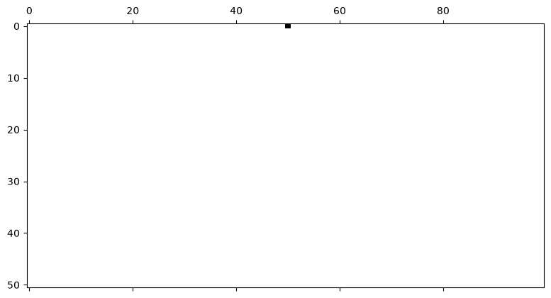
(初期状態の一行目を除いて)常にすべて白となる.
様々なルールへ対応する
Solution to Exercise 2
まず任意のルールに対応できる関数を定義する.
2状態1次元1近傍セルオートマトンのルール総数は 通りあり, セルの状態がからを2進数の8桁にそれぞれ対応させ,各桁の値を遷移後の状態とする.
# 任意のルールに対応できる関数
def rule(rule_num, cell1, cell2, cell3):
    rule_list = []
    mod = rule_num
    for i in range(8):
        k = 7-i
        q, mod = divmod(mod,2**k)
        rule_list.append(q)

    idx = 4*cell1+2*cell2+cell3
    cell2_new = rule_list[7-idx]

    return cell2_new
divmode(p, q)はpをqで割ったときの,と余りを返す関数.
これを使ってルールのセット rule_list を作成する.
各要素はからまでの遷移ルールに対応する.
rule_numにルール番号を与えることで任意のルールに基づいた遷移が実行される.
rule()を使ってシミュレーションをする関数を定義する.
def run_ca(rule_num = 178, n_cells = 100, n_steps = 200):

    cell_list = []
    cell = np.ones(n_cells,dtype=int)

    cell[int(n_cells/2)] = 0
    cell_list.append(cell)
    for t in range(n_steps):
        # -- 状態遷移 --
        cell_tmp = np.ones(n_cells,dtype=int)
        # 境界条件処理その1
        cell_tmp[0] = rule(rule_num, cell[n_cells-1],cell[0],cell[1])
        # メイン
        for i in range(1,n_cells-1,1):
            cell_tmp[i] = rule(rule_num, cell[i-1],cell[i],cell[i+1]);
        # 境界条件処理その2
        cell_tmp[n_cells-1] = rule(rule_num, cell[n_cells-2],cell[n_cells-1],cell[0]);

        # 情報の更新
        cell = np.copy(cell_tmp)

        cell_list.append(cell)

    return cell_list
これを使ったルール0を実行する.
cell_list = run_ca(rule_num = 0, n_cells = 100, n_steps = 50)

plt.figure(dpi=300)
plt.matshow(cell_list[:], cmap="binary")
<Figure size 1920x1440 with 0 Axes>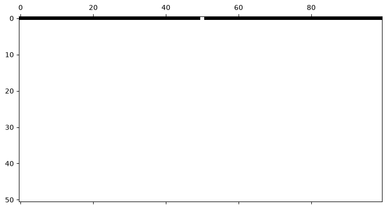
Solution to Exercise 3
ルール90(クラス2)
# ルール90
cell_list = run_ca(rule_num = 90, n_cells = 200, n_steps = 100)

plt.figure(dpi=300)
plt.matshow(cell_list[:], cmap="binary")
<Figure size 1920x1440 with 0 Axes>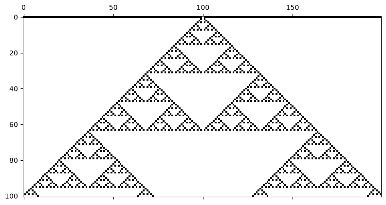
ルール30(クラス3)
# ルール30
cell_list = run_ca(rule_num = 30, n_cells = 200, n_steps = 100)

plt.figure(dpi=300)
plt.matshow(cell_list[:], cmap="binary")
<Figure size 1920x1440 with 0 Axes>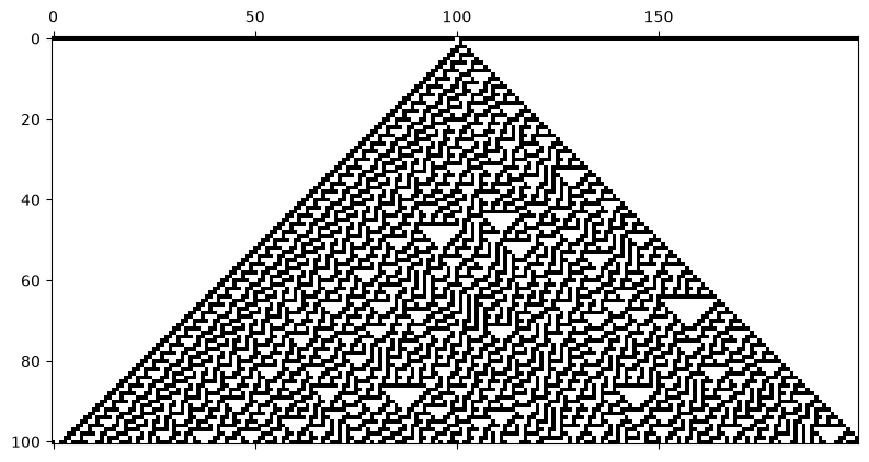
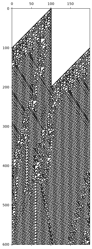
ルール110(クラス4)
# ルール178
cell_list = run_ca(rule_num = 110, n_cells = 200, n_steps = 600)

plt.figure(dpi=300)
plt.matshow(cell_list[:], cmap="binary")
<Figure size 1920x1440 with 0 Axes>