02 連続モデルの数値解と解析解

連続時間の指数増殖モデル $\frac{dx}{dt} = ax$ とロジスティック成長モデル $\frac{dx}{dt} = r(1 - x/K) x$ をオイラー法 (Euler method)で数値的に解き，解析解 (analytical solution)と比較する．

指数増殖とロジスティック成長モデルの解析解¶

指数増殖モデル（解析解）¶

指数増殖モデル $\frac{dx}{dt} = a x$ の解析解は $x(t) = x_0 e^{at}$ になる．増殖率 $a$ はマルサス係数 (Malthusian coefficient)と呼ばれる．

# 02-01. 指数増殖（解析解）
import math

import matplotlib.pyplot as plt

初期値 $x_0 = 10$ ，増殖率 $a = 0.2$ ，刻み幅 $\Delta t = 0.1$ で $t = 0$ から $t = 100$ まで計算する．

a = 0.2
x0 = 10
dt = 0.1

t_list = []
x_list = []
for i in range(1001):
    t = dt * i
    x = x0 * math.exp(a * t)
    t_list.append(t)
    x_list.append(x)

plt.plot(t_list, x_list)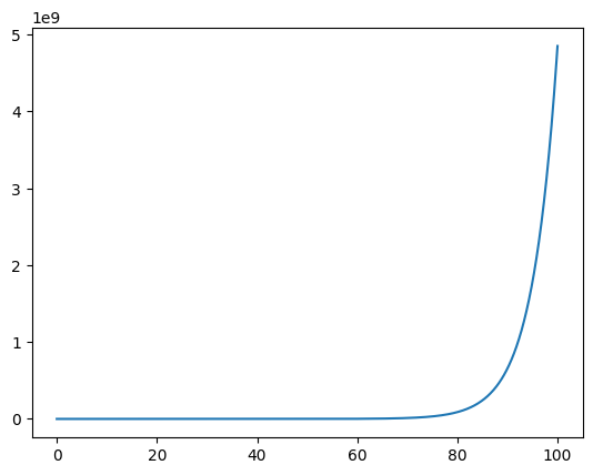

# 02-02. ロジスティック成長（解析解）
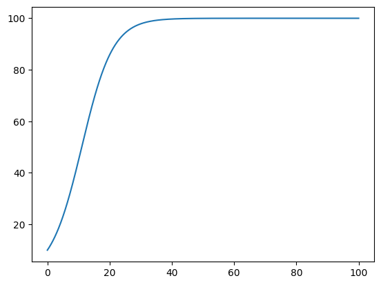
# 指数増殖のプログラムを参考に自分で考えてみてください

ロジスティック成長モデル（解析解）¶

Solution to Exercise 1

r = 0.2
K = 100
x0 = 10
dt = 0.1

t_list = []
x_list = []
for i in range(1001):
    t = dt * i
    x = K / (1 + ((K - x0) / x0) * math.exp(-r * t))
    t_list.append(t)
    x_list.append(x)

plt.plot(t_list, x_list)
plt.title("Logistic growth (analytical)")
plt.xlabel("Time (t)")
plt.ylabel("Pop. size (x)")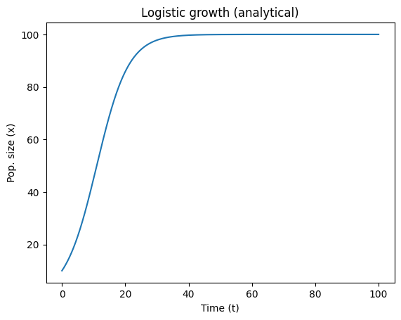

オイラー法による数値解¶

指数増殖（数値解）¶

オイラー法では $x_{t+\Delta t} = x_t + a x_t \, \Delta t$ で次の時刻の値を逐次計算する．離散モデルの実装とほとんど同じかたちになる．

# 02-03. 指数増殖（数値解）
a = 0.2
x0 = 10

dt = 0.1

t = 0
x = x0
t_list = [t]
x_list = [x]
for i in range(1000):
    t = dt * (i + 1)
    x = x + a * x * dt

    t_list.append(t)
    x_list.append(x)

plt.plot(t_list, x_list)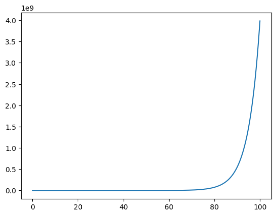

解析解と数値解の比較¶

同じパラメータで解析解と数値解を計算し，1つの図に重ねて誤差の出方を観察する．

# 02-04. 指数増殖（解析解と数値解の比較）
a = 0.2
x0 = 10
t_end = 100

dt_a = 0.1
i_end_a = int(t_end / dt_a)

dt_n = 0.1
i_end_n = int(t_end / dt_n)

# 解析解
x_a_list = []
t_a_list = []
for i in range(i_end_a):
    t = dt_a * i
    x = x0 * math.exp(a * t)
    t_a_list.append(t)
    x_a_list.append(x)

# 数値解
t = 0
x = x0
t_n_list = [t]
x_n_list = [x]
for i in range(i_end_n):
    t = dt_n * (i + 1)
    x = x + a * x * dt_n
    t_n_list.append(t)
    x_n_list.append(x)

# 可視化
plt.plot(t_a_list, x_a_list)
plt.plot(t_n_list, x_n_list)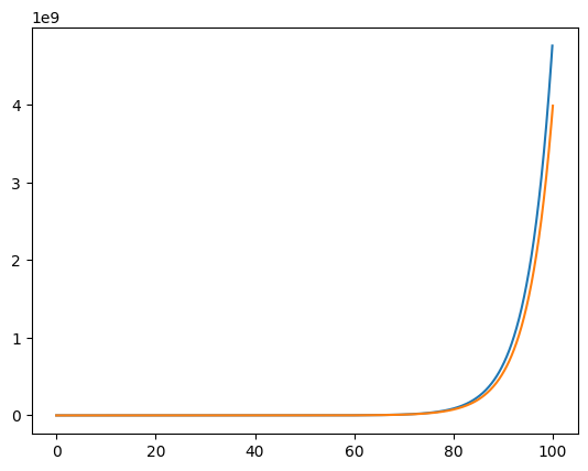

ロジスティック成長モデル（数値解）¶

# 02-05. ロジスティック成長（数値解）
# 指数増殖のプログラムを参考に自分で考えてみてください

Solution to Exercise 2

まずは，オイラー法により，ロジスティック成長モデル $\frac{dx}{dt} = rx(1 - x/K)$ を離散化しよう．

離散化できたら，その更新式を使ってシミュレーションする．

r = 0.2
K = 100
x0 = 10

dt = 0.1

t = 0
x = x0
t_list = [t]
x_list = [x]
for i in range(1000):
    t = dt * (i + 1)
    x = x + r * x * (1 - x / K) * dt

    t_list.append(t)
    x_list.append(x)

plt.plot(t_list, x_list)