07-02 Raupのモデル
対数らせんと可視化
02-01. 対数らせん
# 02-01. 対数らせん
import numpy as np


def logSpiral(a, r0, theta):
    """対数螺旋

    対数螺旋の座標値を返す関数

    Args:
        a: 対数螺旋の拡大率
        r0: 動径の初期値
        theta: 回転角

    Returns:
        x, y: 対数螺旋上の座標値

    """
    r = r0 * np.exp(a * theta)
    x = r * np.cos(theta)
    y = r * np.sin(theta)

    return (x, y)
02-02. 対数螺旋のプロット
# 02-02. 対数螺旋のプロット
import matplotlib.pyplot as plt
# パラメータの設定
r0 = 1
a = 0.2
theta = np.linspace(0, 8 * np.pi, 1000)
# 座標値の計算
x, y = logSpiral(a, r0, theta)# プロット
plt.figure(dpi=200)
plt.axes().set_aspect("equal")
plt.plot(x, y)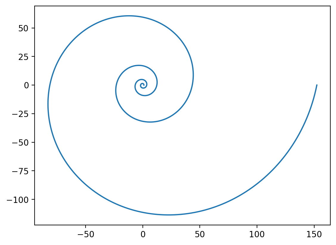
Raupのモデル
02-03. Raupのモデル
# 02-03. Raupのモデル
def raup_model(W, T, D, theta, phi):
    """Raupのモデル

    Raupのモデルに基づき殻表面の座標(x, y, z)を計算する.

    Args:
        W: 螺層拡大率
        T: 転移率(殻の高さ)
        D: 巻軸からの相対的距離(臍の大きさ)
        theta: 成長に伴う回転角
        phi: 殻口に沿った回転角

    Returns:
        x, y, z: 殻表面のx座標,y座標,z座標の
        それぞれの座標値(の配列)

    """
    w = W ** (theta / (2 * np.pi))
    x = w * (2 * D / (1 - D) + 1 + np.cos(phi)) * np.cos(theta)
    y = -w * (2 * D / (1 - D) + 1 + np.cos(phi)) * np.sin(theta)
    z = -w * (2 * T * (D / (1 - D) + 1) + np.sin(phi))
    return (x, y, z)
02-04. Raupのモデルのプロット
# 02-04. Raupのモデルのプロット
import plotly.graph_objs as go
# Raupモデルに基づく殻表面座標の計算
W = 10**0.2
T = 1
D = 0.2
theta_range = np.linspace(0, 8 * np.pi, 800)
phi_range = np.linspace(0, 2 * np.pi, 60)
theta, phi = np.meshgrid(theta_range, phi_range)
x, y, z = raup_model(W, T, D, theta, phi)# プロット
fig = go.Figure(go.Surface(x=x, y=y, z=z, showscale=False))
fig.update_layout(scene={"aspectmode": "data"})
fig.show()Loading...
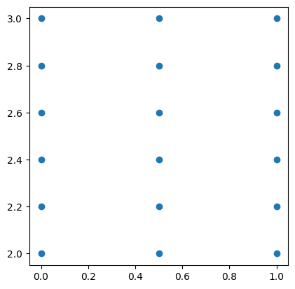
meshgrid
# meshgrid
import matplotlib.pyplot as plt
import numpy as np

a = np.linspace(0, 1, 3)
b = np.linspace(2, 3, 6)
mesh = np.meshgrid(a, b)
x, y = np.meshgrid(a, b)

print(mesh)

plt.axes().set_aspect("equal")
plt.scatter(x, y)
(array([[0. , 0.5, 1. ],
[0. , 0.5, 1. ],
[0. , 0.5, 1. ],
[0. , 0.5, 1. ],
[0. , 0.5, 1. ],
[0. , 0.5, 1. ]]), array([[2. , 2. , 2. ],
[2.2, 2.2, 2.2],
[2.4, 2.4, 2.4],
[2.6, 2.6, 2.6],
[2.8, 2.8, 2.8],
[3. , 3. , 3. ]]))