05-02 ロトカ-ヴォルテラ モデル
ロトカ-ヴォルテラ モデルのシミュレーションとプロット
02-01. 被食-捕食系
# 02-01. 被食-捕食系
import matplotlib.pyplot as plt
# モデルのパラメータ
a = 2.0
b = 3.0
c = 1.0
d = 2.0
# 初期値
x = 0.4
y = 0.4
t = 0.0
# 時間の設定
dt = 0.0001
t_end = 10
i_end = int(t_end / dt) + 1
t_list = [t]
x_list = [x]
y_list = [y]
for i in range(i_end):
t = dt * (i + 1)
x_new = x + dt * (a - b * y) * x
y_new = y + dt * (c * x - d) * y
x = x_new
y = y_new
t_list.append(t)
x_list.append(x)
y_list.append(y)# 時間発展のプロット
plt.plot(t_list, x_list)
plt.plot(t_list, y_list)
plt.legend(["Prey", "Predator"], loc="upper right")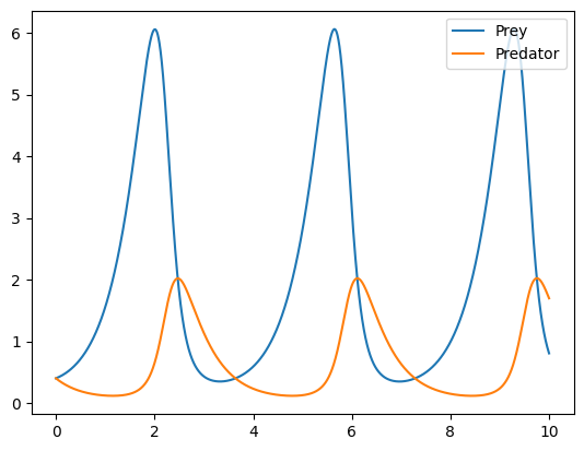
02-02. 相図 被食-捕食系
# 02-02. 相図 被食-捕食系
plt.plot(x_list, y_list)
plt.xlabel("Prey")
plt.ylabel("Predator")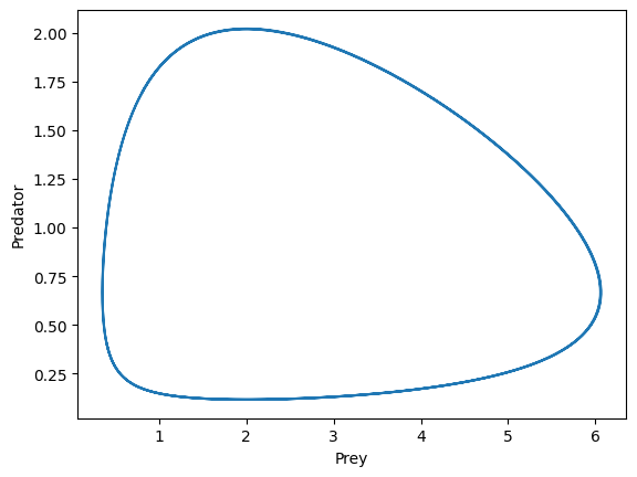
02-03. 競争系
Solution to Exercise 1
例は以下の通り.
# 02-03. 競争系
# モデルのパラメータ
a = 2.0
b = 3.0
c = 1.0
d = 2.0
e = 0.4
f = 2.2

# 初期値
x = 0.15
y = 0.1
t = 0.0

# 時間の設定
dt = 0.0001
t_end = 10
i_end = int(t_end / dt) + 1

t_list = [t]
x_list = [x]
y_list = [y]
for i in range(i_end):
    t = dt * (i + 1)
    x_new = x + dt * (a * x - b * x * x - c * x * y)
    y_new = y + dt * (d * y - e * x * y - f * y * y)
    x = x_new
    y = y_new

    t_list.append(t)
    x_list.append(x)
    y_list.append(y)
計算結果をプロットする.
# 時間発展のプロット
plt.plot(t_list, x_list)
plt.plot(t_list, y_list)
plt.legend(["Sp. 1", "Sp. 2"], loc="upper right")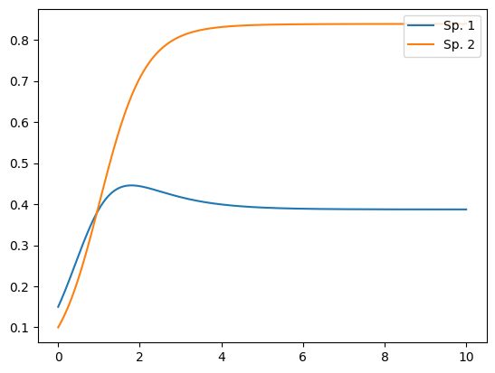
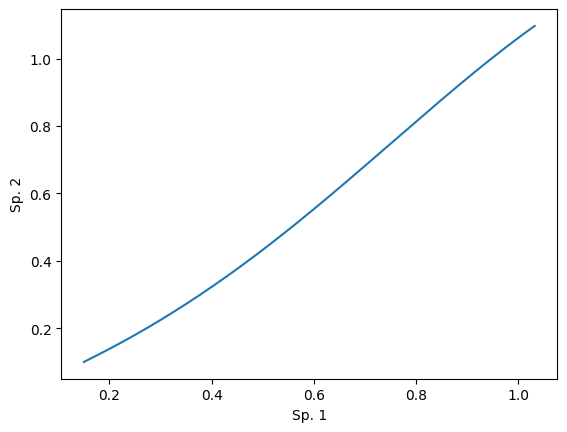
# 相図のプロット
plt.plot(x_list, y_list)
plt.xlabel("Sp. 1")
plt.ylabel("Sp. 2")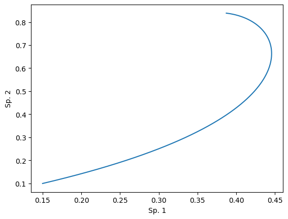
02-04. 共生系
Solution to Exercise 2
例は以下の通り.
# 02-04. 共生系
# モデルのパラメータ
a = 2.0
b = 3.0
c = 1.0
d = 2.0
e = 0.4
f = 2.2

# 初期値
x = 0.15
y = 0.1
t = 0.0

# 時間の設定
dt = 0.0001
t_end = 10
i_end = int(t_end / dt) + 1

t_list = [t]
x_list = [x]
y_list = [y]
for i in range(i_end):
    t = dt * (i + 1)
    x_new = x + dt * (a * x - b * x * x + c * x * y)
    y_new = y + dt * (d * y + e * x * y - f * y * y)
    x = x_new
    y = y_new

    t_list.append(t)
    x_list.append(x)
    y_list.append(y)
計算結果をプロットする.
# 時間発展のプロット
plt.plot(t_list, x_list)
plt.plot(t_list, y_list)
plt.legend(["Sp. 1", "Sp. 2"], loc="upper right")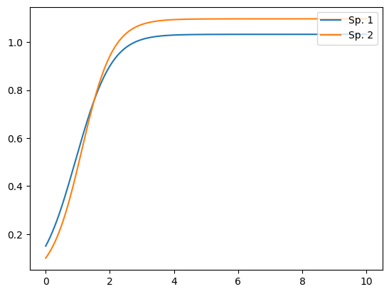
# 相図のプロット
plt.plot(x_list, y_list)
plt.xlabel("Sp. 1")
plt.ylabel("Sp. 2")